In the Data
tab, in the Menu bar, click
on the Conditional Formatting button
(![]() ).
).
The Conditional Formatting pane is displayed with the Conditional Format Options button selected.
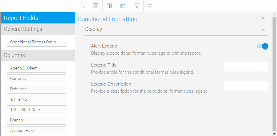
Optional. In the Display section, define the following general settings:
Display option |
Description |
| Alert Legend | Use the toggle switch to display/hide a legend with the conditional formatting rules. |
| Legend Title | Enter the title of the conditional formatting legend. |
| Legend Description | Enter the description of the conditional formatting legend. |
In the Columns section, click on the column for which you want to create a conditional rule.
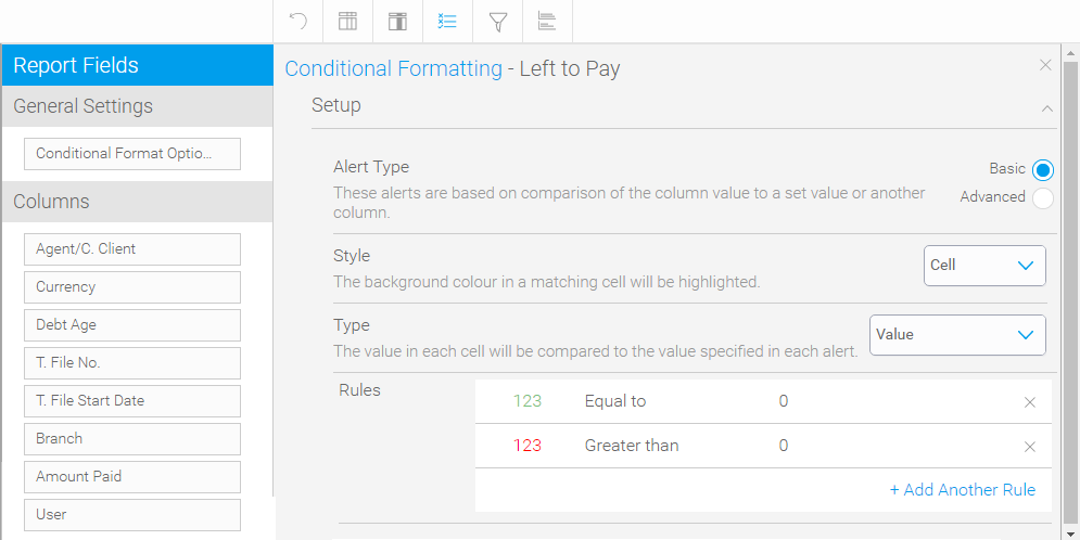
A new Setup section is displayed.
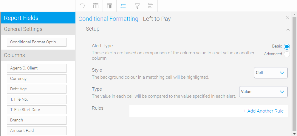
In the Alert Type field, leave the basic option selected.
In the Style field, select one of the following options:
Bar: The value in a matching cell will be displayed as a bar. Only available for measurable columns.
Cell: The background color in a matching cell will be highlighted.
Icon: The text in a matching cell will be replaced with an icon you select from a predefined list of icons.
Measure columns only. In the Type field, select one of the following options:
Value: The value in each cell is compared to the value you define in the rules (see below). For example, Amount is greater than 0.
Compare Column: The value in each cell is compared to the value in a different column (see below). For example, the Supplier Price is compared to the Net to Remit.
Percentage of Column: The value in each cell is compared to a percentage of a different column. For example, the Supplier Price is compared to 95% of the Net to Remit.
Percentage of Total: The value in each cell is compared to the total value of the column as a percentage. For example, each cell that is less than 5% of the total Amount column.
Percentage of Max: The value in each cell is compared to a percentage of the maximum value of the cell. For example, the maximum transaction fee amount is 100 USD. Cells with a 95 USD transaction fee are marked in green.
If you selected to compare to a different column, in the Target field, select the column you wish to compare to.
In the Rules field, click +Add Another Rule.
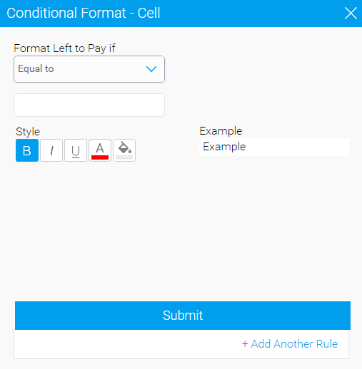
A Conditional Format - Cell dialog box is displayed.
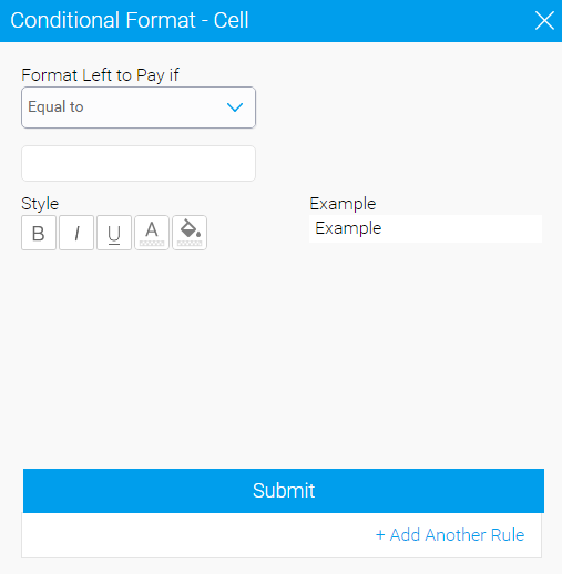
In the Format Amount If field, select the condition for formatting the contents of the cell. For example: Equal To or Greater Than.
Enter the amount or percentage the cell should be compared to.
Date columns only. In the Dynamic Date field, select whether the condition applies to a dynamic date or static date.
If enabled, in the Current Date field define to when the cell should be compared. For example, Current Date + 3 Weeks.
If disabled, select the static date to which the cell should be compared. For example, 25/01/2020.
In the Style section, define how the cell will be formatted if the condition is met. For example, the cell background is highlighted green and the contents are bolded.
Click Submit.
|
The Style options are determined according to the option you selected in the Style field (Step 5). |
To add another rule, click + Add Another Rule.
When you close the Conditional Formatting pane, the rule will be saved.

 Click here for a detailed example